The transformer architecture is the neural network design behind almost every modern large language model. It replaced recurrent networks for two reasons: attention lets each token draw on other tokens directly, and training runs in parallel on modern hardware. This guide builds the transformer architecture step by step with worked numbers and a few lines of code, and ends with the interview questions that come up about it, including why generation happens one token at a time when training is parallel.
If you're new to LLMs, read how large language models work first.
The big picture: a transformer in one sentence
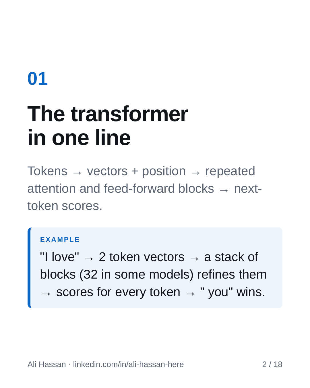
In a decoder-only model, the kind behind most chat assistants, the flow is:
token embeddings + position information → a stack of repeated blocks (attention + feed-forward) → a projection onto the vocabulary → next-token scores.
For example, take the input "I love". The tokenizer produces two token IDs, and each becomes a vector. A stack of blocks (32 in some models, more or fewer in others) refines those vectors. The final vector at the last position is projected onto the vocabulary to give a score for every possible next token, and " you" might come out on top.
Each block refines every token's representation a little. Roughly, early blocks pick up surface patterns and later blocks build more abstract features, though real models don't follow that rule strictly.
Step 1: tokens become vectors
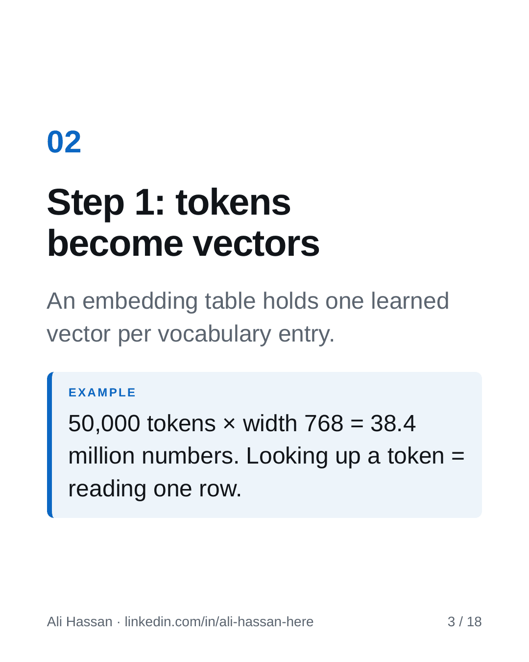
The model can't do arithmetic on token IDs, so the first layer is an embedding table with one learned vector per vocabulary entry.
Worked example: with a vocabulary of 50,000 tokens and a model width of 768, the embedding table holds 50,000 × 768 = 38.4 million numbers. Looking up a token means reading one row of that table.
These vectors are learned during training. Tokens used in similar contexts tend to end up with related vectors, which lets later layers work with meaning instead of raw IDs.
Step 2: adding position information
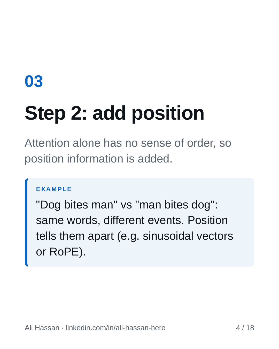
Attention on its own treats the input as a set, with no sense of order. Order matters, though: "Dog bites man" and "man bites dog" contain the same words and describe different events.
So the model adds position information. The original Transformer added fixed sinusoidal position vectors to the token embeddings. Many modern models use rotary position embeddings (RoPE), which encode position by rotating the query and key vectors inside attention. Either way, each token's representation now carries both what it is and where it is.
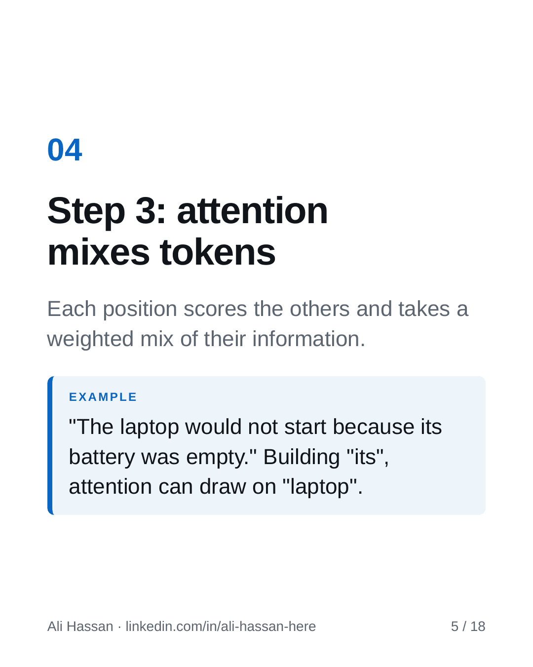
Step 3: attention mixes information between positions
Attention is where tokens exchange information. For each position, the model scores how relevant each allowed position is, then takes a weighted mix of their information.
Consider the sentence "The laptop would not start because its battery was empty." When the model builds a representation for "its", attention can pull in information from "laptop", which helps it track what "its" refers to. In real models this is spread across many heads and layers, so don't expect one clean link per word.
Each block usually has several attention heads working in parallel, so different heads can pick up different kinds of relationships. The next post in this series covers the attention formula in detail.
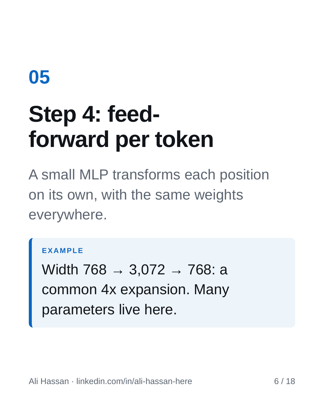
Step 4: the feed-forward network transforms each position
After attention mixes information across positions, a feed-forward network (a small multi-layer perceptron) transforms each position on its own, applying the same weights to every position.
A common pattern expands the width and then projects back. For example, with a model width of 768, the feed-forward layer might go 768 → 3,072 → 768, a 4x expansion. A large share of a Transformer's parameters sit in these layers.
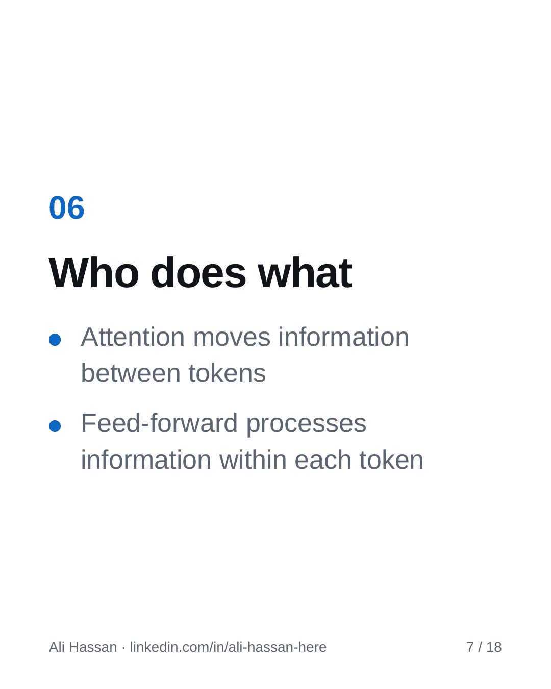
An easy way to remember the division of labour: attention moves information between tokens, and the feed-forward network processes information within each token.
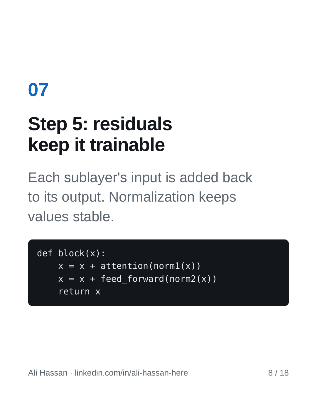
Step 5: residual connections and normalization
Deep stacks are hard to train. Residual connections add each sublayer's input back to its output, which gives information and gradients a direct path around the sublayer. Layer normalization keeps the values in a stable range. In code, a common pre-norm block looks like this:
def transformer_block(x):
    x = x + attention(layer_norm_1(x))
    x = x + feed_forward(layer_norm_2(x))
    return x
The x = x + ... lines are the residual paths. Without them, very deep networks are much harder to optimize, although residuals still need careful initialization and normalization alongside them.
Encoder, decoder and encoder-decoder transformer architecture
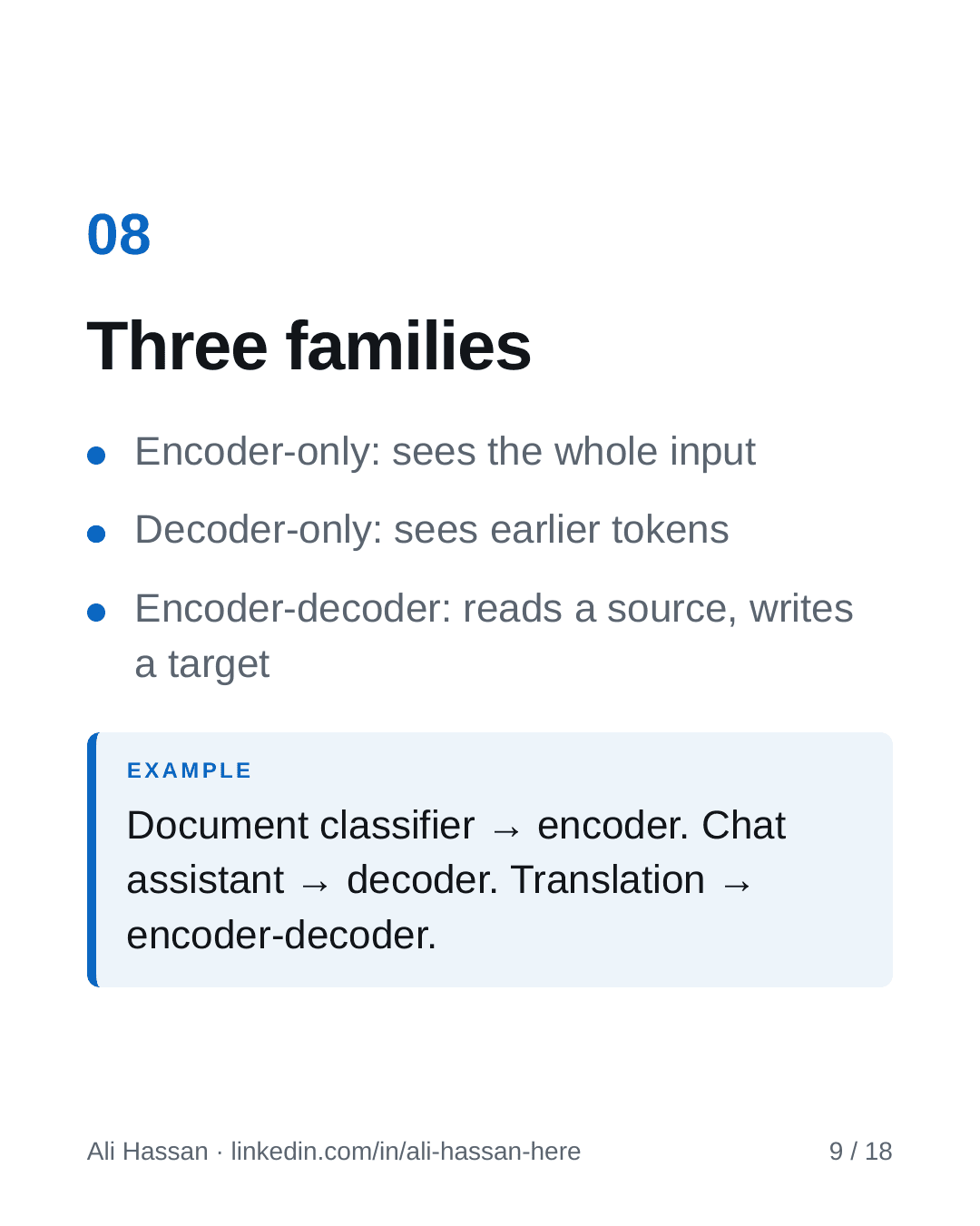
The same building blocks are arranged into three families:
| Family | What each token can see | Typical uses |
|---|---|---|
| Encoder-only | The whole input | Classification, retrieval, embeddings |
| Decoder-only | Only earlier tokens | Text generation, chat assistants |
| Encoder-decoder | Encoder reads the source; decoder generates with cross-attention to it | Translation, summarization |
For instance, a document classifier can use an encoder's representation of the whole text, a chat assistant typically uses a decoder, and a translation model can use an encoder-decoder design. The families describe typical designs; decoder models are also used for classification, for example.
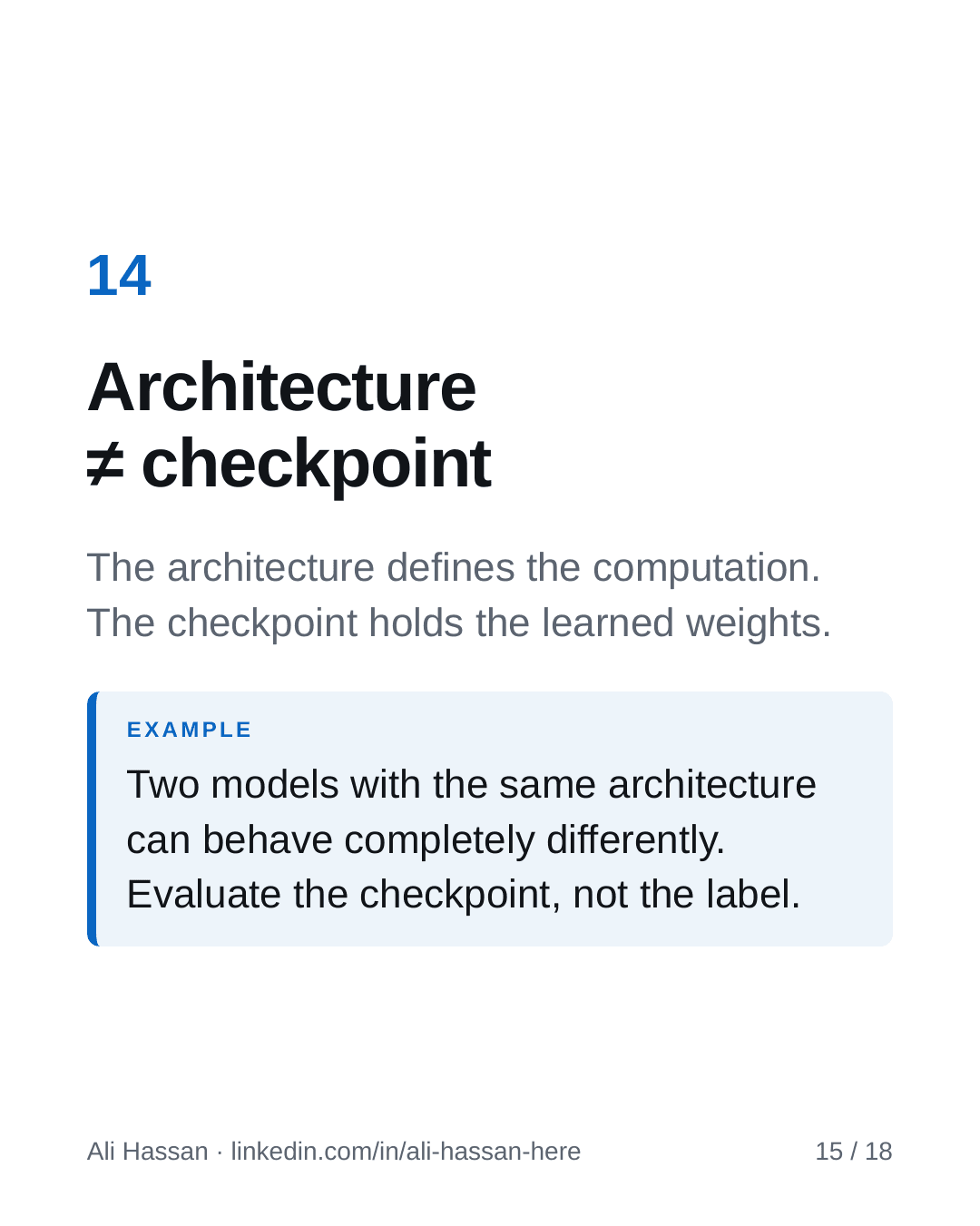
The architecture name also leaves a lot out. A checkpoint is the set of learned weights, and the architecture defines the computation that uses them. Two models with the same architecture can behave very differently, so evaluate the checkpoint itself.
The causal mask
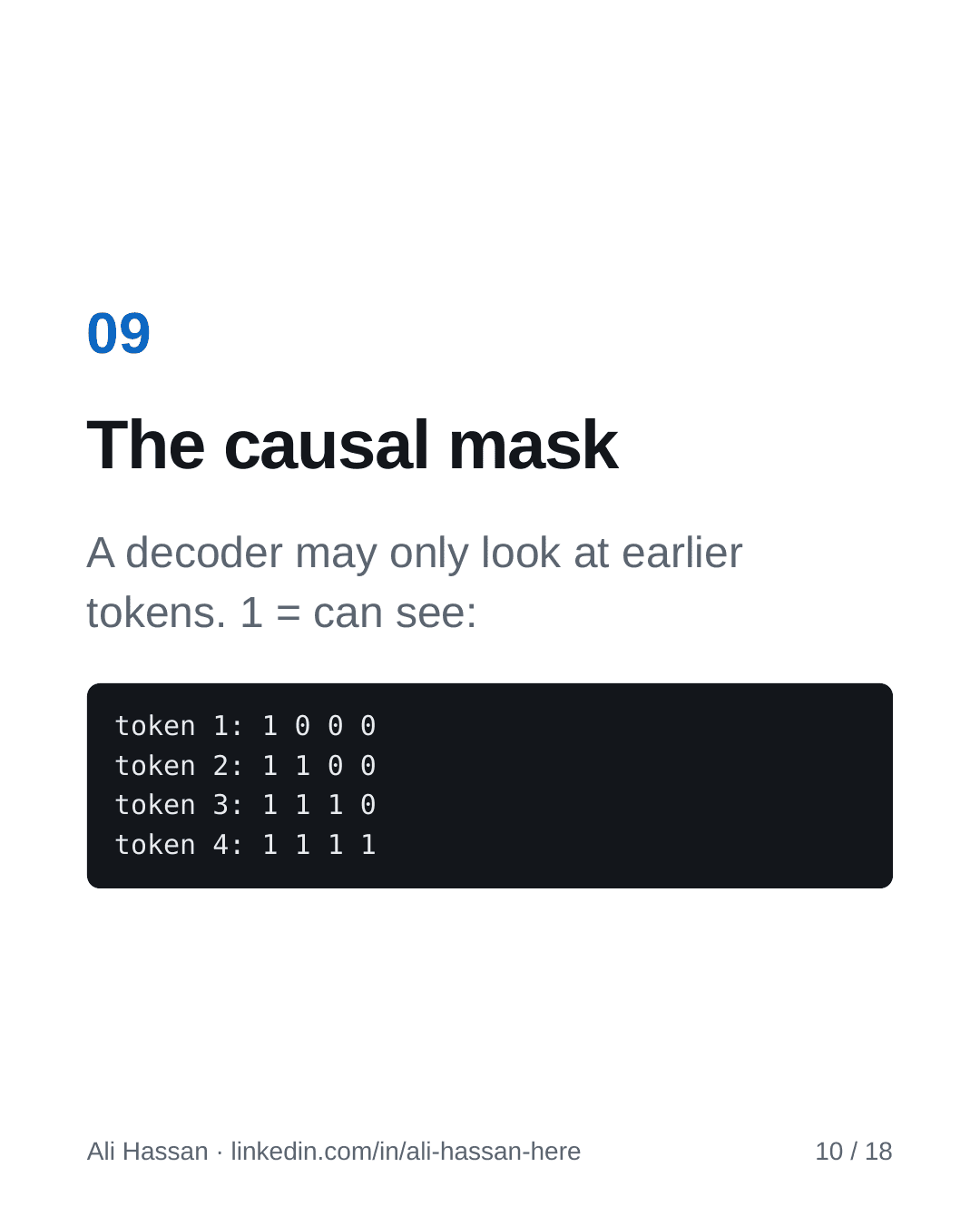
A decoder must not peek at future tokens, or it would learn to cheat during training. The causal mask enforces this: position i may attend only to positions up to i.
Here is the mask for four tokens, where 1 means "can see":
token 1: 1 0 0 0
token 2: 1 1 0 0
token 3: 1 1 1 0
token 4: 1 1 1 1
If future tokens were visible during causal training, the model could use information it won't have at generation time, and training metrics would look excellent while it learned the wrong task.
Why training is parallel but generation is sequential
This part of the transformer architecture is a common interview question.
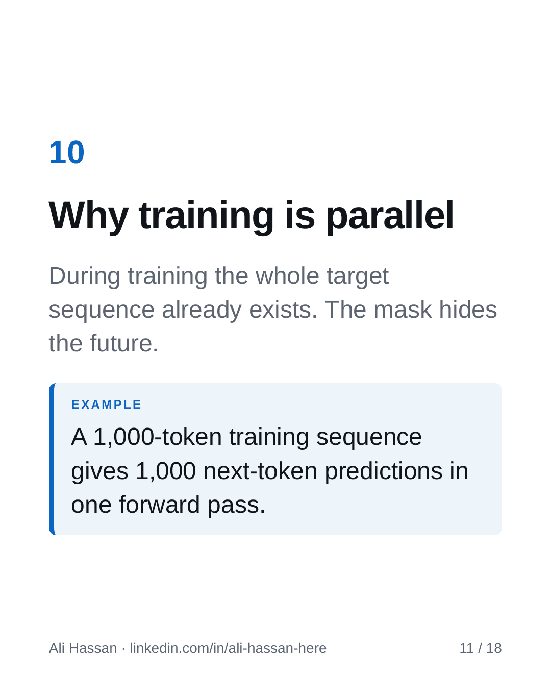
During training the whole target sequence already exists. The causal mask hides the future from each position, so the model can compute predictions for every position at once: a 1,000-token training sequence yields 1,000 next-token predictions from a single forward pass.
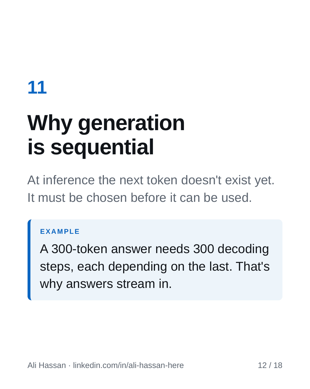
At inference time the next token doesn't exist yet. The model has to choose token 1 before it can use it to choose token 2, so a 300-token answer needs 300 decoding steps, each depending on the one before. That's why a chat assistant streams its answer piece by piece. Inference engines cache earlier keys and values so they don't recompute everything at each step, and a later post in this series covers that KV cache.
If an interviewer asks why generation is slower than training per sequence, explain both halves: the causal mask lets training process all positions together, while generation has to produce tokens one after another.
Why transformers replaced RNNs
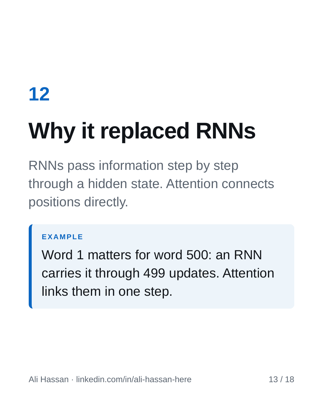
Recurrent neural networks (RNNs) process a sequence one step at a time and pass information forward through a hidden state. That causes two problems.
Long-range information is hard to keep. Suppose word 1 matters for word 500: an RNN must carry that information through 499 sequential updates, while attention connects the two positions directly.
Training also can't run in parallel across positions. Each step depends on the previous hidden state, so an RNN can't process a sequence's positions at the same time the way a Transformer can during training.
Direct links between distant positions, combined with parallel training, made it practical to train much larger models on much more data.
The cost of attention
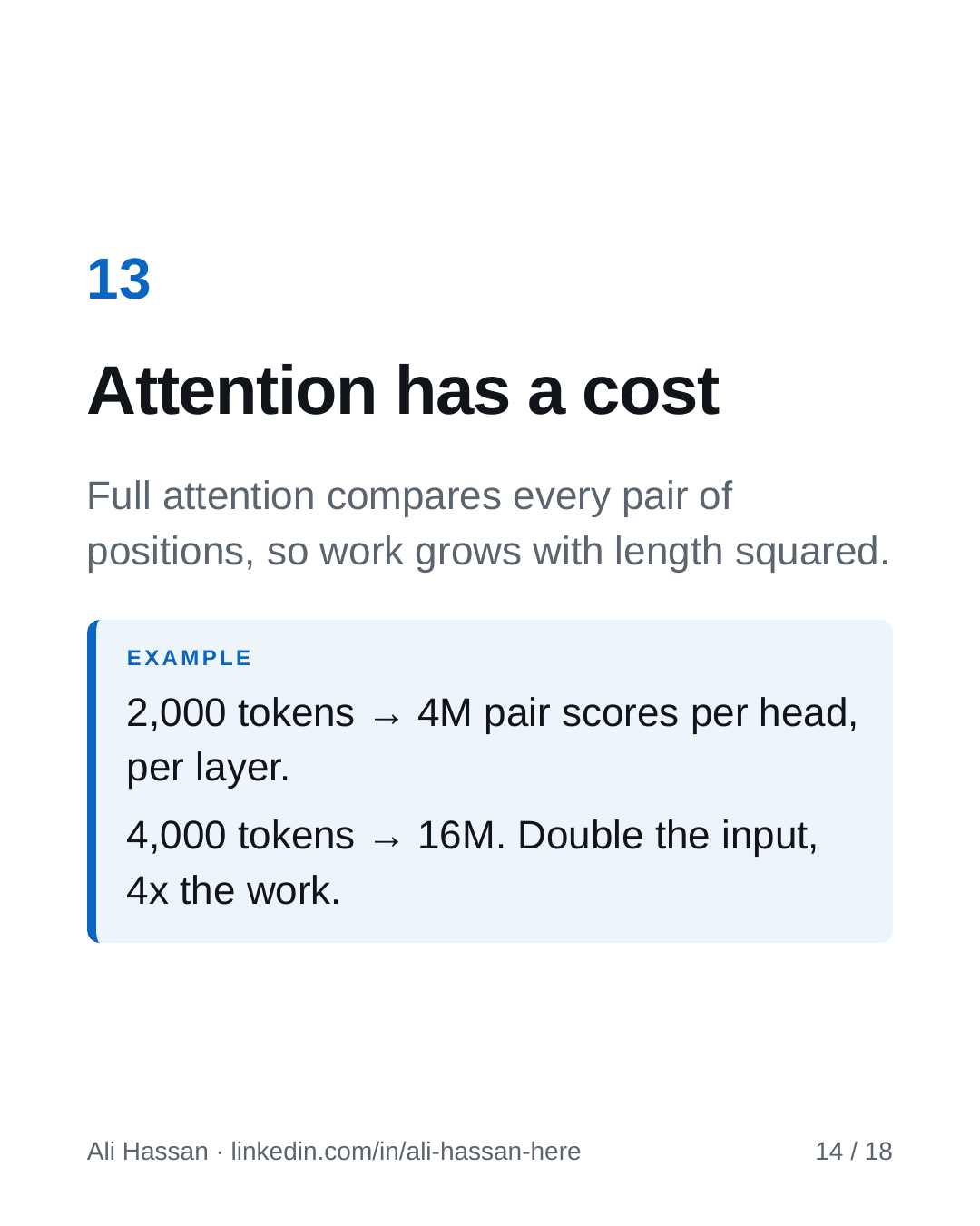
Standard full attention computes interactions between every pair of positions, so the work grows with the square of the sequence length.
Let's say you double the input. At 2,000 tokens, one attention head in one layer computes 4 million pairwise scores; at 4,000 tokens it computes 16 million. Efficient attention kernels reduce memory traffic, but they don't remove the quadratic arithmetic, which is one reason long contexts are expensive.
Common misconceptions
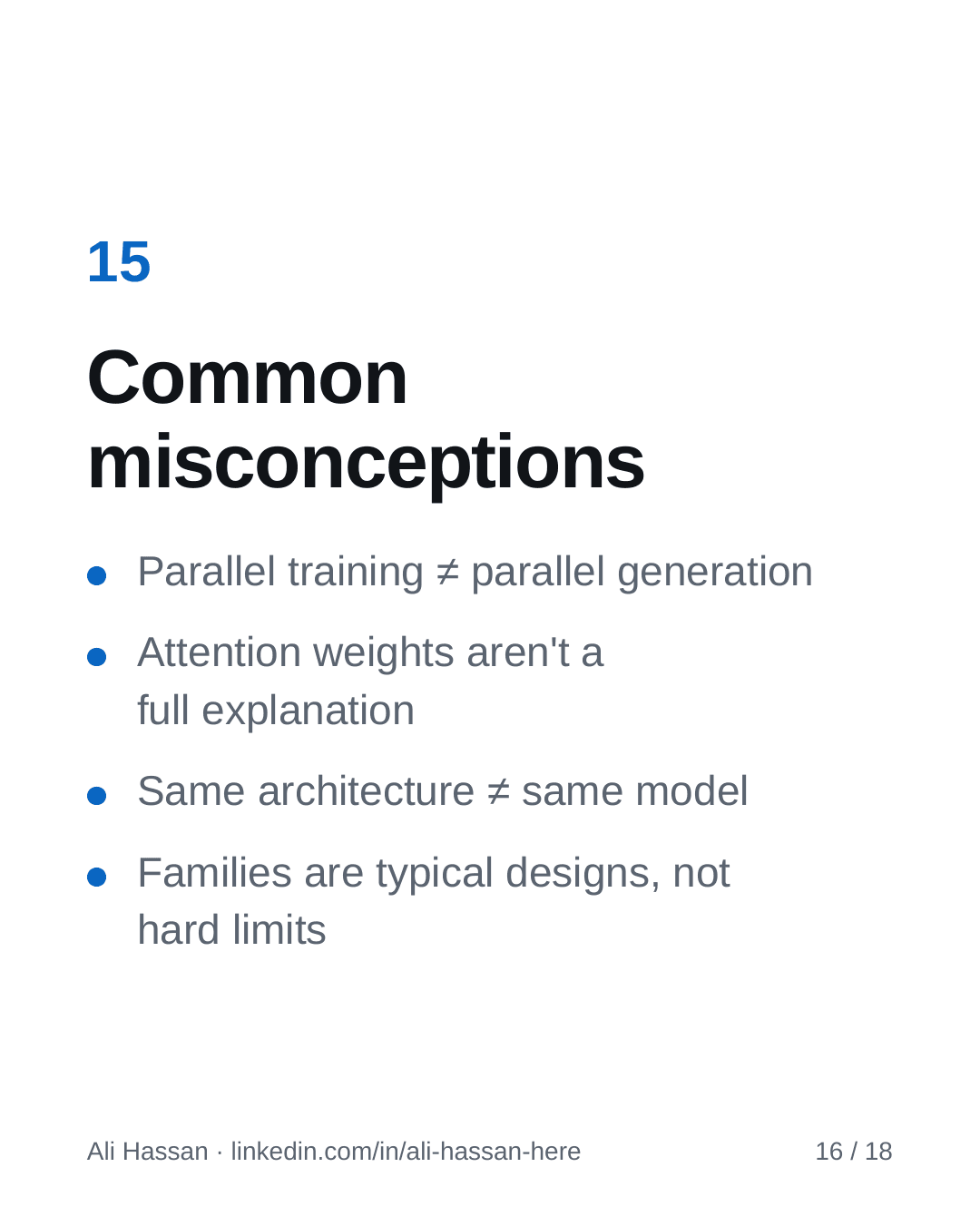
- Parallel training does not mean parallel generation. Generation still happens token by token.
- Attention weights help you inspect behaviour, but they aren't a complete causal explanation of an answer.
- Two models with the same architecture can behave differently, because the weights decide behaviour.
- The three families describe typical designs, not hard limits on what a model can do.
Frequently asked questions
Why did attention help replace recurrent sequence processing?
It creates direct interactions between distant positions and supports parallel computation across positions during training. Recurrent networks propagate information through sequential state updates.
Why are residual connections useful?
They give information and gradients a path around each sublayer, which makes deep networks easier to optimize. They don't remove the need for careful initialization and normalization.
Why is generation slower than parallel training per sequence?
In ordinary autoregressive generation, later tokens don't exist yet. The model must select each token before it can condition on it for the next step, while training sees the whole sequence at once.
What is the difference between an architecture and a checkpoint?
The architecture defines the computation, and the checkpoint contains the learned weights. Select and evaluate the complete checkpoint, not just the architecture name.
Key takeaways
- A decoder-only transformer architecture turns tokens into vectors, adds position, refines them through attention and feed-forward blocks, and scores the next token.
- Attention moves information between tokens, and the feed-forward network processes each token on its own.
- Residual connections and normalization make deep stacks trainable.
- The causal mask makes training parallel, while missing future tokens make generation sequential.
- Attention cost grows with the square of the sequence length.
A good exercise is to draw one decoder block and label the input, output, causal mask, residual paths, normalization and vocabulary head. For more depth, read the original paper, Attention Is All You Need, and the Hugging Face course chapter on how Transformers work. The next post in this series covers the attention mechanism step by step.